Data Generation : Botox case study (continuous endpoint)

set.seed(42)

case_study_config <- yaml::yaml.load_file(system.file("conf/case_studies/botox.yml", package = "BExTE"))
format_case_study_config(case_study_config)

Case Study Configuration
Parameter	Value
General
Name	Botox
Control	Placebo
Summary Measure Likelihood	normal
Theta 0	0
Endpoint	continuous
Null Space	left
Sampling Approximation	FALSE
Target
Control	130
Treatment	126
Total	256
Treatment Effect	0.1
Standard Error	0.1
Source
Control	235
Treatment	233
Total	468
Treatment Effect	0.2
Standard Error	0.1

Generation of aggregate data

source_data <- SourceData$new(case_study_config)

drift <- 0.4
target_sample_size_per_arm <- 100

target_data <- TargetDataFactory$new()
target_data <- target_data$create(source_data = source_data, case_study_config = case_study_config, target_sample_size_per_arm = target_sample_size_per_arm, treatment_drift = drift, summary_measure_likelihood = source_data$summary_measure_likelihood)

n_replicates <- 10000
data <- target_data$generate(n_replicates = n_replicates)
print(data[1:10,])

##    treatment_effect_estimate treatment_effect_standard_error
## 1                  0.8097144                       0.1648389
## 2                  0.5136186                       0.1501266
## 3                  0.6555475                       0.1506688
## 4                  0.6968085                       0.1599049
## 5                  0.6618406                       0.1345548
## 6                  0.5837662                       0.1598121
## 7                  0.8312163                       0.1689636
## 8                  0.5855201                       0.1607539
## 9                  0.9087566                       0.1455753
## 10                 0.5904067                       0.1382090
##    sample_size_per_arm standard_deviation
## 1                  100           1.648389
## 2                  100           1.501266
## 3                  100           1.506688
## 4                  100           1.599049
## 5                  100           1.345548
## 6                  100           1.598121
## 7                  100           1.689636
## 8                  100           1.607539
## 9                  100           1.455753
## 10                 100           1.382090

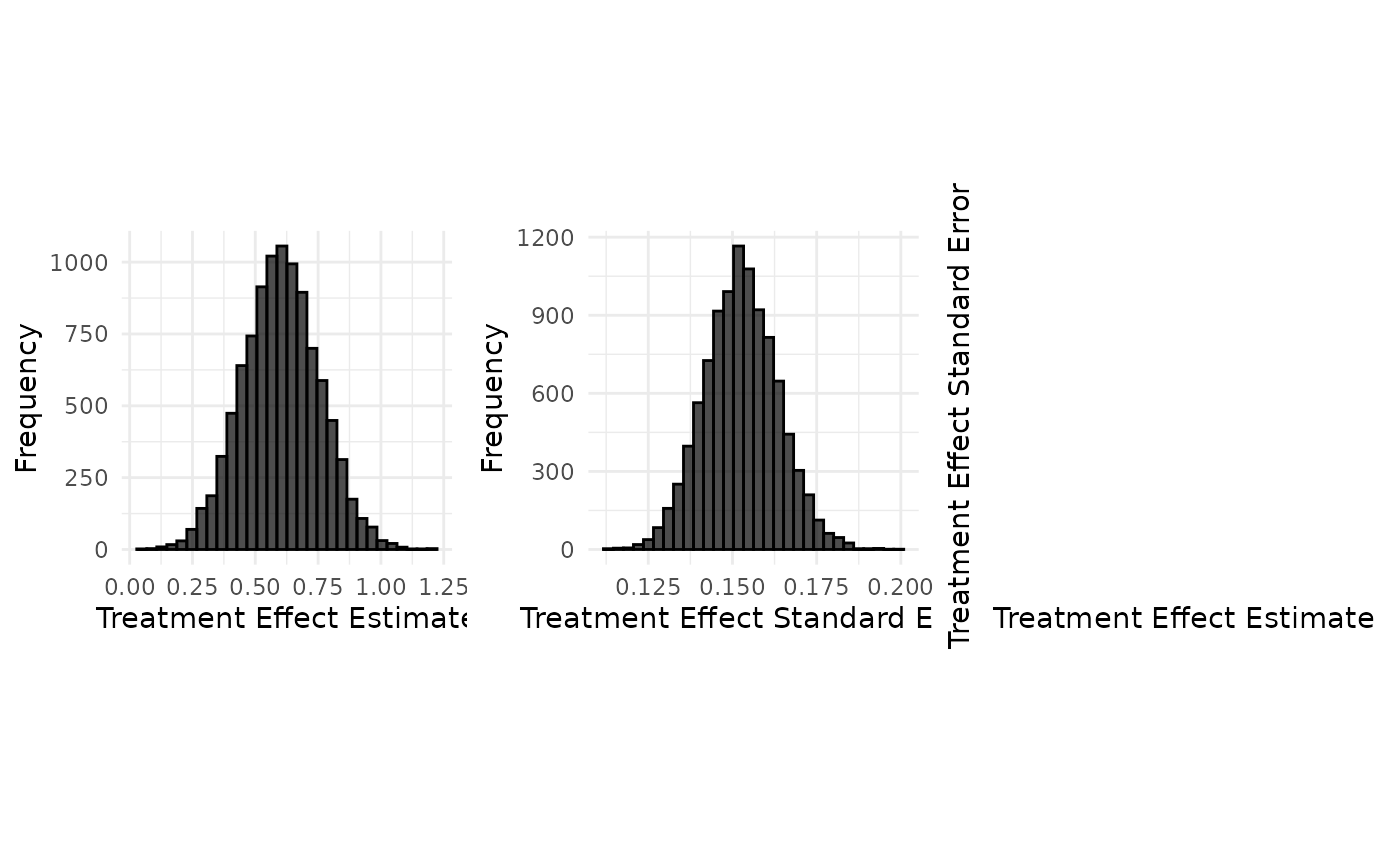
target_data$plot_sample(data)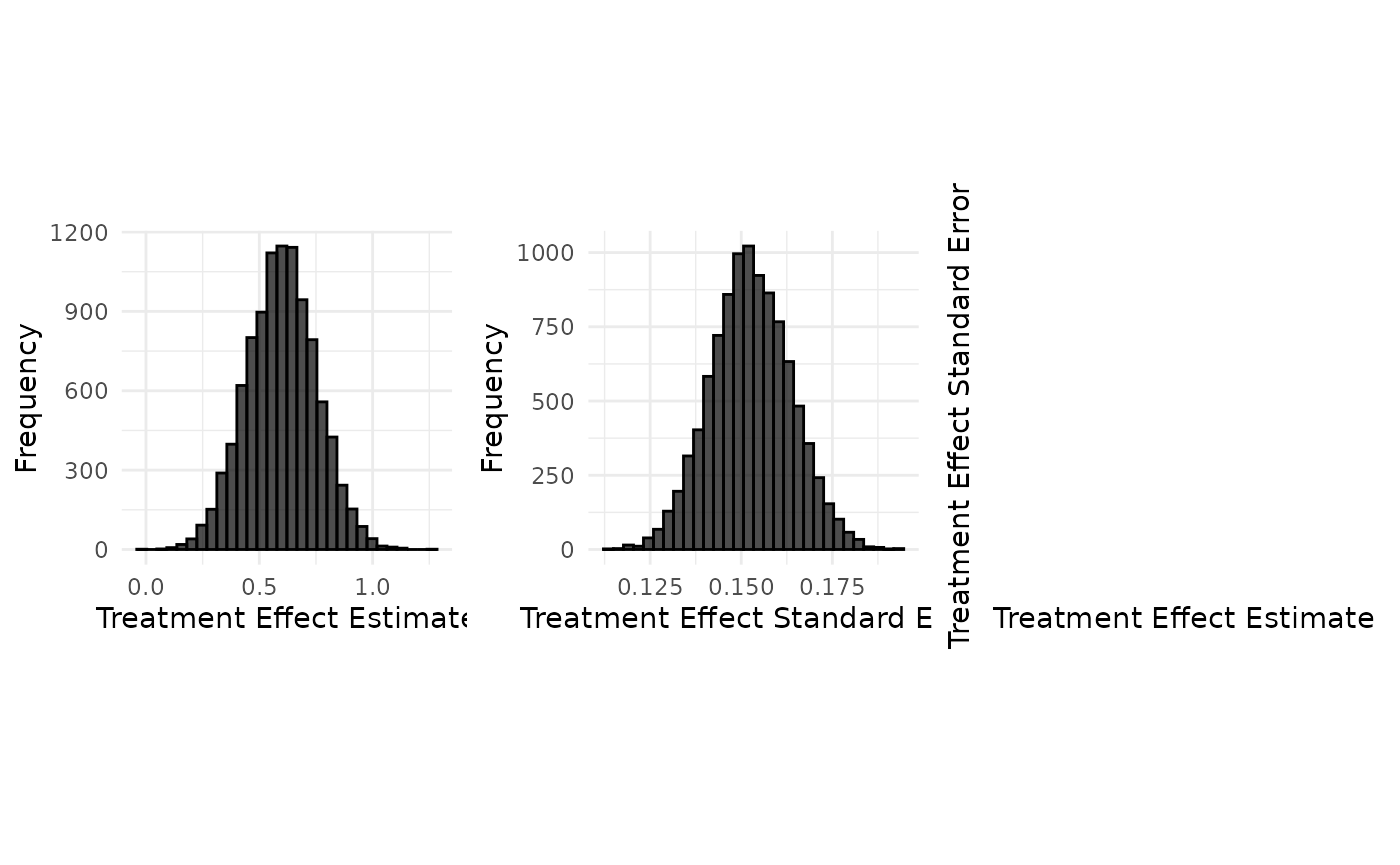

Sampling standard deviation and the known-variance assumption

The target study’s sampling standard deviation is not set in the case study configuration. It is derived from the source study:

$\sigma_T = r \, \mathrm{SE}_S \sqrt{n_S},$

where $\mathrm{SE}_S$ is the standard error of the source treatment effect, $n_S$ the source’s equivalent sample size per arm and $r$ the target_to_source_std_ratio (1 by default; a scenarios configuration can vary it through target_to_source_std_ratio_range). With $r = 1$ , the target data are generated with the sample standard deviation of the source study, i.e. of the adults: the simulation assumes children’s outcomes are as variable as adults’.

target_data$standard_deviation holds this true value $\sigma_T$ :

target_data$standard_deviation

## [1] 1.529692

source_data$standard_error * sqrt(source_data$equivalent_source_sample_size_per_arm)

## [1] 1.529692

Each replicate carries its own estimate instead, drawn around $\sigma_T$ :

summary(data$standard_deviation)

##    Min. 1st Qu.  Median    Mean 3rd Qu.    Max. 
##   1.136   1.452   1.525   1.526   1.601   1.932

The analysis methods only see these per-replicate estimates. The Bayesian methods use a normal likelihood whose variance is the replicate’s squared standard error, treated as if it were known exactly, so the uncertainty in the variance estimate is ignored. The true $\sigma_T$ is only used to generate data and for design-stage quantities such as the analytical power of the reference test.

Implementation details

read_function_code(sample_aggregate_normal_data)

## sample_aggregate_normal_data <- function (mean, variance, n_replicates, n_samples_per_arm) 
## {
##     sample_mean <- rnorm(n_replicates, mean = mean, sd = sqrt(variance/n_samples_per_arm))
##     if (n_samples_per_arm > 1) {
##         degrees_of_freedom <- n_samples_per_arm - 1
##         sample_variance <- variance * rchisq(n_replicates, df = degrees_of_freedom)/degrees_of_freedom
##     }
##     else {
##         sample_variance <- rep(NA_real_, n_replicates)
##     }
##     sample_standard_error <- sqrt(sample_variance/n_samples_per_arm)
##     samples <- data.frame(treatment_effect_estimate = sample_mean, 
##         treatment_effect_standard_error = sample_standard_error, 
##         sample_size_per_arm = n_samples_per_arm, standard_deviation = sqrt(sample_variance))
##     return(samples)
## }

samples <- sample_aggregate_normal_data(
  mean = target_data$treatment_effect,
  variance = target_data$standard_deviation^2,
  n_replicates = n_replicates,
  n_samples_per_arm = target_data$sample_size_per_arm
)

target_data$plot_sample(samples)

2026-10-03

Generation of aggregate data

Sampling standard deviation and the known-variance assumption

Implementation details