Data Generation : Teriflunomide case study (time-to-event endpoint)

2026-10-03

Teriflunomide case study

Sources: Bovis et al (2022)

The source study is the pooled analysis of the adult TEMSO and TOWER trials of 14 mg teriflunomide; Table 4 of the TOWER paper by Confavreux et al (2014) reports it. The target study is a paediatric trial inspired by the TERIKIDS design. The endpoint is the time to first relapse.

The source treatment effect is the pooled log hazard ratio $\widehat{\theta}_S = \log(\widehat{HR}_S) = -0.393$, with $\widehat{\sigma}_{\theta_S} = 0.081$. The target treatment effect is $\theta_T = \widehat{\theta}_S + \delta$, where $\delta$ is the drift.

set.seed(42)

config_path <- system.file("conf/case_studies/teriflunomide.yml", package = "BExTE")
case_study_config <- yaml::yaml.load_file(config_path)
format_case_study_config(case_study_config)

Case Study Configuration
Parameter	Value
General
Name	Teriflunomide
Summary Measure Likelihood	normal
Theta 0	0
Endpoint	time_to_event
Null Space	right
Sampling Approximation	FALSE
Target
Control (Target)	57
Treatment (Target)	109
Total (Target)	166
Treatment Effect (Target)	-0.415515443961666
Standard Error (Target)	0.266828713056808
Maximum follow-up time (Target)	1.846154
Accrual period (Target)	3.41
Follow-up after recruitment (Target)	0.923077
Weibull shape (Target)	0.72
Weibull relapse-free probability (Target)	0.442
Source
Control (Source)	752
Treatment (Source)	731
Total (Source)	1483
Treatment Effect (Source)	-0.393
Standard Error (Source)	0.081
Maximum follow-up time (Source)	2

The target trial design

In the original TERIKIDS design every participant could be followed for up to 96 weeks, so accrual would not affect the follow-up distribution. To study the effect of staggered accrual we use a modified fixed-calendar design: the maximum individual follow-up stays at $L = 96$ weeks, but the database is closed $F = 48$ weeks after the end of recruitment.

Patients enter over an accrual period of $A = 3.41$ years, with calendar entry times $R_i \sim \mathcal{U}(0, A)$. The database closes at $C = A + F$, so the administrative censoring time of patient $i$ is

$$C_i = \min\{L,\ A + F - R_i\}.$$

Control-arm heterogeneity is $\kappa = \log \lambda_T^{(c)} - \log \lambda_S^{(c)}$, so that $\lambda_T^{(c)} = \lambda_S^{(c)} e^{\kappa}$ and $\lambda_T^{(t)} = \lambda_T^{(c)} e^{\theta_T}$. In the package $\kappa$ is the control_drift of a scenario and $\delta$ is its drift.

Independent loss to follow-up is $D_i \sim \operatorname{Exp}(\lambda_D)$ with $\lambda_D = -\log(1 - p_D)/L$ for a prespecified probability $p_D$ of being lost over $L$. The observed follow-up time and the event indicator are

$$X_i = \min(T_i, D_i, C_i), \qquad \Delta_i = \mathbb{1}\{T_i \leq D_i,\ T_i \leq C_i\}.$$

design <- case_study_config$target
L <- design$max_follow_up_time
A <- design$accrual_period
Fu <- design$final_follow_up

# Only patients recruited before A + F - L are followed for the full L.
c(max_follow_up = L, accrual = A, final_follow_up = Fu,
  proportion_with_full_follow_up = (A + Fu - L) / A)

##                  max_follow_up                        accrual 
##                      1.8461540                      3.4100000 
##                final_follow_up proportion_with_full_follow_up 
##                      0.9230770                      0.7293029

Creating the target data

source_data <- SourceData$new(case_study_config)

drift <- 0.2 # delta
control_drift <- 0 # kappa
treatment_drift <- drift + control_drift

target_sample_size_per_arm <- 185

target_data <- TargetDataFactory$new()
target_data <- target_data$create(
  source_data = source_data,
  case_study_config = case_study_config,
  target_sample_size_per_arm = target_sample_size_per_arm,
  control_drift = control_drift,
  treatment_drift = treatment_drift,
  summary_measure_likelihood = source_data$summary_measure_likelihood,
  dropout_probability = 0.05,
  event_time_distribution = "exponential"
)

c(theta_T = target_data$treatment_effect,
  control_rate = target_data$control_rate,
  treatment_rate = target_data$treatment_rate)

##        theta_T   control_rate treatment_rate 
##     -0.1930000      0.5340000      0.4402734

The arm rates follow from $\kappa$ and $\theta_T$:

read_function_code(rate_from_drift_logRR)

## rate_from_drift_logRR <- function (arm_drift, source_rate) 
## {
##     return(source_rate * exp(arm_drift))
## }

Aggregate data generation

Generation of aggregate data without sampling approximation

Usage

n_replicates <- 2000
data <- target_data$generate(n_replicates = n_replicates)
head(data)

##   treatment_effect_estimate treatment_effect_standard_error sample_size_per_arm
## 1                -0.3517472                       0.1432327                 185
## 2                -0.1546573                       0.1438881                 185
## 3                -0.2028978                       0.1417119                 185
## 4                -0.3259558                       0.1493049                 185
## 5                 0.1238848                       0.1392157                 185
## 6                -0.0580501                       0.1434024                 185
##   standard_deviation
## 1           1.948176
## 2           1.957089
## 3           1.927490
## 4           2.030767
## 5           1.893538
## 6           1.950483

target_data$plot_sample(data)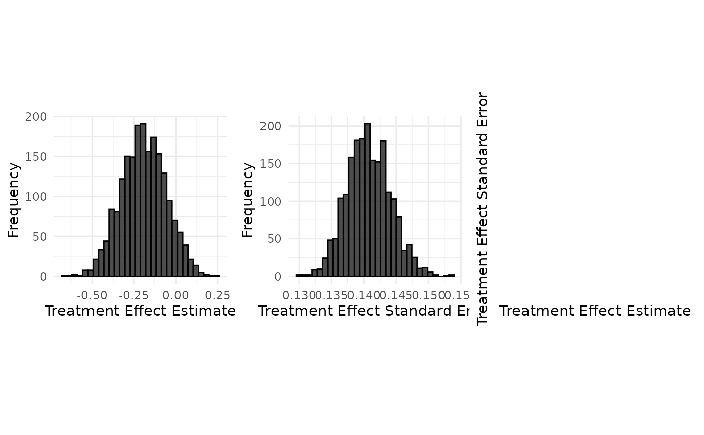

Implementation details

Under the primary proportional-hazards model the time to first relapse is exponential, $T_i \mid Z_i = a \sim \operatorname{Exp}(\lambda_T^{(a)})$. Each simulated trial is analysed with a Cox proportional-hazards model $h_i(t) = h_0(t)\exp\{\beta \mathbb{1}(Z_i = t)\}$, and $\widehat{\theta}_T = \widehat{\beta}$ with $\widehat{\sigma}_{\theta_T} = \operatorname{SE}(\widehat{\beta})$ are passed to the Bayesian borrowing procedures as in the other case studies.

Fitting one survival::coxph() per replicate would be far too slow for the simulation grid, so the package solves the two-sample Cox model directly. With a single binary covariate the risk set at an event time is described entirely by the numbers still at risk in each arm, $(n_0, n_1)$, so the score and observed information reduce to

$$U(\beta) = d_1 - \sum_{\text{events}} \frac{n_1 e^{\beta}}{n_0 + n_1 e^{\beta}}, \qquad I(\beta) = \sum_{\text{events}} \frac{n_0 n_1 e^{\beta}}{(n_0 + n_1 e^{\beta})^2},$$

which a few Newton steps solve for every replicate at once. Event times are continuous, so ties have probability zero and this agrees with coxph() to machine precision. The patient-level version below is what the vectorised code computes:

simulate_one_trial <- function(n_per_arm, control_rate, treatment_rate,
                               L, A, Fu, dropout_rate) {
  n <- 2 * n_per_arm
  arm <- rep(c(0, 1), each = n_per_arm)
  rate <- ifelse(arm == 0, control_rate, treatment_rate)

  entry <- runif(n, 0, A)
  administrative <- pmin(L, A + Fu - entry)
  event_time <- rexp(n, rate = rate)
  dropout <- if (dropout_rate > 0) rexp(n, rate = dropout_rate) else Inf

  data.frame(
    time = pmin(event_time, dropout, administrative),
    status = as.integer(event_time <= dropout & event_time <= administrative),
    arm = arm
  )
}

dropout_rate <- -log1p(-0.05) / L

set.seed(123)
trial <- simulate_one_trial(
  n_per_arm = target_sample_size_per_arm,
  control_rate = target_data$control_rate,
  treatment_rate = target_data$treatment_rate,
  L = L, A = A, Fu = Fu, dropout_rate = dropout_rate
)

fit <- survival::coxph(survival::Surv(time, status) ~ arm, data = trial)
c(estimate = unname(coef(fit)), standard_error = unname(sqrt(diag(vcov(fit)))))

##       estimate standard_error 
##     -0.2119895      0.1411929

The package reproduces that fit exactly:

vectorised <- BExTE:::fit_two_sample_cox(
  time = matrix(trial$time, nrow = 1),
  event = matrix(trial$status, nrow = 1),
  arm = trial$arm
)
c(estimate = vectorised$estimate, standard_error = vectorised$standard_error)

##       estimate standard_error 
##     -0.2119895      0.1411929

Averaged over replicates, the estimates recover $\theta_T$ and the reported standard errors match their spread:

c(theta_T = target_data$treatment_effect,
  mean_estimate = mean(data$treatment_effect_estimate, na.rm = TRUE),
  mean_standard_error = mean(data$treatment_effect_standard_error, na.rm = TRUE),
  observed_spread = sd(data$treatment_effect_estimate, na.rm = TRUE))

##             theta_T       mean_estimate mean_standard_error     observed_spread 
##          -0.1930000          -0.1924182           0.1407653           0.1340475

Weibull sensitivity analysis

As a sensitivity analysis, event times are generated from a Weibull proportional-hazards model with conditional survival function $S(t \mid Z_i) = \exp\{-(t/b_c)^q \exp(\theta_T Z_i)\}$, where $q$ is the common shape parameter and $b_c$ the control-arm scale. This implies a hazard ratio of $\exp(\theta_T)$. We use $q = 0.72$, based on the aggregate TERIKIDS relapse-free probabilities. The control scale is calibrated to reproduce the reported 96-week relapse-free probability $S_c(L) = 0.442$, giving

$$b_c = L / [-\log\{S_c(L)\}]^{1/q} = 2.45 \text{ years},$$

and the treatment-arm scale is $b_t = b_c \exp(-\theta_T/q)$. The exponential model is recovered when $q = 1$.

Because $\exp(\kappa)$ multiplies the control hazard, and multiplying a Weibull hazard by a constant divides its scale by that constant raised to $1/q$, control heterogeneity enters as $b_c(\kappa) = b_c \exp(-\kappa/q)$.

weibull_data <- TargetDataFactory$new()$create(
  source_data = source_data,
  case_study_config = case_study_config,
  target_sample_size_per_arm = target_sample_size_per_arm,
  control_drift = control_drift,
  treatment_drift = treatment_drift,
  summary_measure_likelihood = source_data$summary_measure_likelihood,
  dropout_probability = 0.05,
  event_time_distribution = "weibull"
)

c(shape = weibull_data$weibull_shape,
  control_scale = weibull_data$weibull_scale,
  relapse_free_at_L = 1 - pweibull(L, weibull_data$weibull_shape,
                                   weibull_data$weibull_scale))

##             shape     control_scale relapse_free_at_L 
##           0.72000           2.44676           0.44200

Note that the two data-generating models are deliberately not nested: the exponential arm is calibrated on the source placebo relapse rate, the Weibull arm on the aggregate relapse-free probability, so they do not coincide at $\kappa = 0$.

weibull_samples <- weibull_data$generate(n_replicates = n_replicates)
c(theta_T = weibull_data$treatment_effect,
  mean_estimate = mean(weibull_samples$treatment_effect_estimate, na.rm = TRUE))

##       theta_T mean_estimate 
##    -0.1930000    -0.1876292

Generation of aggregate data with sampling approximation

Usage

approximate_config <- case_study_config
approximate_config$sampling_approximation <- TRUE

approximate_data <- TargetDataFactory$new()$create(
  source_data = source_data,
  case_study_config = approximate_config,
  target_sample_size_per_arm = target_sample_size_per_arm,
  control_drift = control_drift,
  treatment_drift = treatment_drift,
  summary_measure_likelihood = source_data$summary_measure_likelihood
)

samples <- approximate_data$generate(n_replicates = n_replicates)

approximate_data$plot_sample(samples)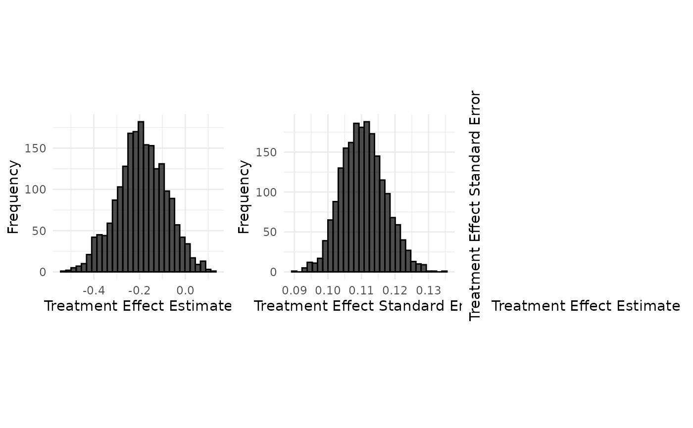

Implementation details

It may be simpler for evaluating the OCs to sample the summary data from a normal distribution directly, instead of sampling data using the true data generating process. This branch keeps the simpler follow-up model in which every patient is observed for max_follow_up_time: it samples the number of events in each arm from a Poisson distribution, forms $\operatorname{SE}(\log RR) = \sqrt{1/e_c + 1/e_t}$, and draws the summary measure from a normal distribution. It therefore ignores the staggered accrual, the database lock and the loss to follow-up, and is not the design described above.

See Data_generation_botox for details on aggregate normal data generation.