Commensurate Prior
2026-10-03
Source:vignettes/methods/Commensurate_Prior.Rmd
Commensurate_Prior.RmdIntroduction
This vignette describes an implementation of the Commensurate Prior, the location commensurate model of Hobbs et al (2011) without its power parameter. See the Commensurate Power Prior vignette for the variant that carries one.
Set working directory, import functions and configurations
List packages to load, and install them if necessary.
Mathematical description of the model
The source data inform through their own likelihood, undiscounted, and the target parameter is tied to it by a commensurability precision :
where is an initial prior for and
This is the commensurate power prior at : the Beta prior on the power parameter disappears, and with it the second route by which that model adapts the amount of borrowing. Here the borrowing is governed by alone. Small inflates the variance of the prior for and so discounts the source; large pulls towards .
Gaussian case
With a noninformative initial prior and a Gaussian likelihood, integrating out leaves a prior that is normal conditional on :
and equation (9) of Hobbs et al (2011), evaluated at , gives
where , and
Because the posterior is an ordinary conjugate update of a normal
mixture over
,
the simulation does not fit this model with Stan for every replicate:
vectorised_replicate_inference() discretises
on a quadrature rule and updates the whole mixture at once. The Stan
program below remains the reference implementation, and is what
inference() uses for a single data set.
Implementation of the model in Stan
case_study_config <- yaml::yaml.load_file(system.file("conf/case_studies/belimumab.yml", package = "BExTE"))


source_data <- ObservedSourceData$new(case_study_config)
summary_measure_likelihood <- case_study_config$summary_measure_likelihood
endpoint <- case_study_config$endpoint

target_data <- ObservedTargetData$new(treatment_effect_estimate = case_study_config$target$treatment_effect, treatment_effect_standard_error = case_study_config$target$standard_error, target_sample_size_per_arm = as.integer(case_study_config$target$total / 2), summary_measure_likelihood = case_study_config$summary_measure_likelihood)
method_parameters <- list(
  initial_prior = "noninformative", # The posterior for the source data is derived from an uninformative prior, for consistency with the other methods.
  heterogeneity_prior = list(family = "inverse_gamma", alpha = 1 / 3, beta = 1)
  # list(family = "half_normal", std_dev = 5)
  # list(family = "cauchy", location = 0, scale = 10)
)

env = "full"
config_dir <- paste0(system.file(paste0("conf/", env), package = "BExTE"), "/")
mcmc_config <- yaml::read_yaml(paste0(config_dir, "/mcmc_config.yml"))

model <- Model$new()

model <- model$create(
  case_study_config = case_study_config,
  method = "commensurate_prior",
  method_parameters = method_parameters,
  source_data = source_data,
  mcmc_config = mcmc_config
)

print(model$stan_model_code)
## [1] "\n data {\n int<lower=0,upper=2> prior_type; // Type of prior on the commensurability parameter; 0 for inverse_gamma, 1 for half normal, 2 for Cauchy\n int<lower=1> NS; // Number of samples in dataset S\n int<lower=1> NT; // Number of samples in dataset T\n real<lower=0> target_sampling_variance; // Known variance of the target data\n real<lower=0> prior_variance; // Prior variance component\n real source_treatment_effect_estimate; // Estimate from dataset S\n real target_treatment_effect_estimate; // Estimate from dataset T\n real std_dev; // Parameter for the half normal prior\n real location; // Location parameter for the Cauchy prior\n real scale; // Scale parameter for the Cauchy prior\n real alpha; // Parameter for the inverse_gamma prior\n real beta; // Pocation parameter for the inverse_gamma prior\n }\n\n parameters {\n // Sampled on the log scale, which Stan's <lower=0> transform on tau\n // already did internally, so that tau itself is never formed where\n // it would overflow: a Cauchy(0, 30) prior on log(tau) puts about 3%\n // of its mass beyond log(tau) = +-709, the limit of exp().\n real log_tau; // Log commensurability parameter\n real target_treatment_effect; // Target treatment effect\n }\n\n model {\n // Local to the model block, as in the power prior variant, and\n // likewise written in 1 / tau so that they stay finite however\n // large tau grows.\n // Capped so that no product below overflows. The marginal\n // likelihood weights log(tau) < -600 by about exp(-300), so\n // the cap moves no posterior mass that a double can represent.\n real inverse_tau = exp(fmin(-log_tau, 600));\n real u_over_tau = NS * inverse_tau + prior_variance;\n real denominator = NS * target_sampling_variance + NT * u_over_tau;\n real marginal_variance = target_sampling_variance / NT\n + inverse_tau\n + prior_variance / NS;\n\n // Priors\n // Each prior is stated on its own quantity and carried to log_tau\n // by the log Jacobian of that change of variables; constant terms\n // are dropped.\n if (prior_type == 0) {\n // tau^2 ~ InvGamma(alpha, beta). With s = log(tau^2) = 2 * log_tau\n // the density of s is inv_gamma_lpdf(exp(s)) + s, which reduces to\n // -alpha * s - beta * exp(-s); ds / dlog_tau = 2 is constant.\n // Writing it out avoids forming tau^2, which overflows at the\n // log(tau) of about 354 that alpha = 1/1000 reaches.\n target += -2 * alpha * log_tau - beta * exp(-2 * log_tau);\n } else if (prior_type == 1){\n // tau ~ HN(std_dev), plus the log Jacobian of tau = exp(log_tau).\n // The half-normal's normalising constant is fixed by the data.\n target += normal_lpdf(exp(log_tau) | 0, std_dev) + log_tau;\n } else if (prior_type == 2){\n // The prior is on log_tau itself, so there is no Jacobian.\n log_tau ~ cauchy(location, scale);\n }\n\n // Marginal target-data likelihood for the commensurability\n // parameter. With the conditional distribution below this is\n // equation (9) of Hobbs et al. (2011) at gamma = 1. Omitting it\n // would leave tau distributed according to its prior.\n target_treatment_effect_estimate ~ normal(\n source_treatment_effect_estimate,\n sqrt(marginal_variance));\n\n // Numerator and denominator divided by tau, as in the power\n // prior variant.\n target_treatment_effect ~ normal(\n (NS * target_sampling_variance * source_treatment_effect_estimate + NT * u_over_tau * target_treatment_effect_estimate) /\n denominator,\n sqrt(u_over_tau * target_sampling_variance / denominator));\n }\n\n generated quantities {\n real tau = exp(log_tau); // Commensurability parameter\n }\n "
model$inference(target_data)In the inference method, the data are prepared for use with Stan
using the same prepare_data() as the commensurate power
prior - the two Stan programs share a data block:
data <- model$prepare_data(target_data)Then, draws are sampled from the posterior following the configuration specified in mcmc_config.
bayesplot::mcmc_hist(model$fit$draws("target_treatment_effect"), binwidth = 0.001)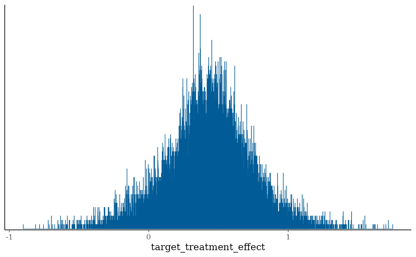
posterior <- model$fit$draws("target_treatment_effect")
bayesplot::color_scheme_set("blue")
bayesplot::mcmc_dens(posterior, pars = c("target_treatment_effect"))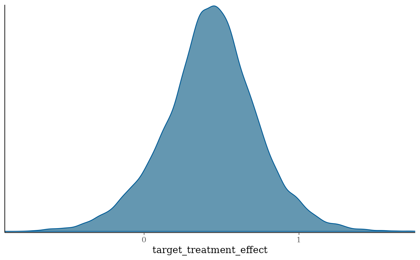
Posterior distribution of the heterogeneity parameter. There is no power parameter to plot alongside it:
posterior <- model$fit$draws("tau")
bayesplot::color_scheme_set("blue")
bayesplot::mcmc_dens(posterior, pars = c("tau"))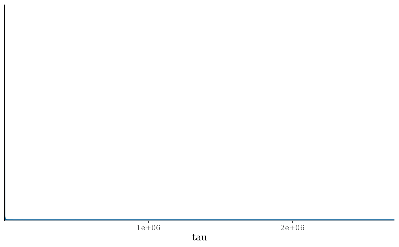
library(posterior)
draws_array <- as_draws_array(model$fit)
library(bayesplot)
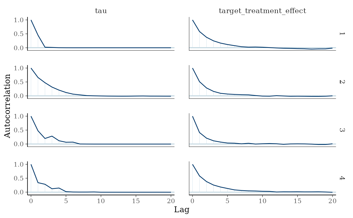
mcmc_trace(draws_array, pars = c("tau", "target_treatment_effect"))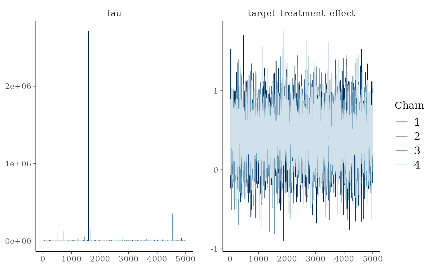
mcmc_diagnostics <- model$fit$diagnostic_summary()

n_draws <- mcmc_config$chain_length * mcmc_config$num_chains

# MCMC Effective Sample Size
mcmc_ess <- bayesplot::neff_ratio(model$fit) * n_draws

mcmc_ess <- mcmc_ess[["target_treatment_effect"]]
print(mcmc_ess)
## [1] 5151.52
rhat_values <- bayesplot::rhat(model$fit)
rhat <- rhat_values["target_treatment_effect"]
print(rhat)
## target_treatment_effect
## 1.000763
# number of divergences reported is the sum of the per chain values
n_divergences <- sum(mcmc_diagnostics$num_divergent)
print(n_divergences)
## [1] 69