Empirical Mixture Prior (Egidi)

2026-10-03

Introduction

This vignette describes an implementation of the data-dependent mixture prior of Egidi, Pauli and Torelli. It uses the same two components as the Robust Mixture Prior, and differs from it in one respect only: the mixture weight is not prespecified, it is selected from the observed target data.

See the Gaussian RMP vignette for the components themselves, which are not changed here. Holding them fixed is what makes a comparison between the two methods a comparison of the weight rule alone.

Mathematical description of the model

Egidi et al. parameterise the mixture by the weight on the weak component:

$$\pi_\psi(\theta_T) = \psi\, q(\theta_T) + (1 - \psi)\, p(\theta_T), \qquad 0 \le \psi \le 1,$$

where $p(\theta_T) = N(\mu_p, \tau_p^2)$ is the informative, source-based component and $q(\theta_T) = N(\mu_q, \tau_q^2)$ is the weak or unit-information component. So $\psi = 0$ means full use of the informative prior and $\psi = 1$ means complete reliance on the weak one.

The Robust Mixture Prior in this package parameterises the same mixture by the weight $w$ on the informative component, so the two conventions are related by

$$w = 1 - \psi.$$

The prior predictive and the conflict $p$-value

For each component $j \in \{p, q\}$, the prior-predictive distribution of the target statistic is

$$m_j(t) = \int f_T(t \mid \theta_T)\, j(\theta_T)\, d\theta_T.$$

With a normal target likelihood $\hat\theta_T \mid \theta_T \sim N(\theta_T, s_T^2)$ this is available in closed form,

$$m_p(t) = N(t \mid \mu_p,\, s_T^2 + \tau_p^2), \qquad m_q(t) = N(t \mid \mu_q,\, s_T^2 + \tau_q^2),$$

and the predictive under the mixture is $m_\psi = \psi m_q + (1 - \psi) m_p$.

The conflict $p$-value is the probability that the prior predictive puts the statistic somewhere at least as improbable as where it landed:

$$P_\psi(t_{\mathrm{obs}}) = \Pr_{T \sim m_\psi}\left\{ m_\psi(T) \le m_\psi(t_{\mathrm{obs}}) \right\}.$$

The inequality is on the density of the complete mixture. Averaging the two component $p$-values is a different quantity as soon as the components have different centres, which in this study is the ordinary case: the informative component sits at the source estimate and the weak one at $\theta_0$.

Two cases are exact. Both ends of the weight range collapse the mixture to a single normal, so

$$P_0 = 2\Phi\!\left(-\frac{|t_{\mathrm{obs}} - \mu_p|}{\sqrt{s_T^2 + \tau_p^2}}\right), \qquad P_1 = 2\Phi\!\left(-\frac{|t_{\mathrm{obs}} - \mu_q|}{\sqrt{s_T^2 + \tau_q^2}}\right),$$

whatever the centres are. And when the centres coincide, $\mu_p = \mu_q$, the mixture predictive is symmetric and decreasing in $|t - \mu|$, so $P_\psi = (1 - \psi) P_p + \psi P_q$ exactly.

Otherwise $P_\psi$ is evaluated by splitting the line into the pieces on which $m_\psi$ is monotone and integrating between the level crossings, each of which is then available in closed form from the component distribution functions.

Selecting the weight

With $\alpha_{\mathrm{PC}} = 0.05$,

$$\hat\psi = \inf\left\{ \psi \in [0, 1] : P_\psi(t_{\mathrm{obs}}) \ge \alpha_{\mathrm{PC}} \right\}.$$

For common-centred components this inverts in closed form:

$$\hat\psi = \begin{cases} 0, & P_p \ge \alpha_{\mathrm{PC}},\\[4pt] \dfrac{\alpha_{\mathrm{PC}} - P_p}{P_q - P_p}, & P_p < \alpha_{\mathrm{PC}} \le P_q,\\[10pt] 1, & P_q < \alpha_{\mathrm{PC}}. \end{cases}$$

In the last case the weak component cannot remove the conflict. The rule still returns $\hat\psi = 1$, but the replicate is flagged with conflict_unresolved = TRUE rather than being reported as a conflict that was resolved.

When the centres differ, $P_\psi$ is not guaranteed to be monotone in $\psi$: with the components this study uses it can fall before it rises when the observed statistic sits near the informative centre. The infimum is therefore found by scanning upwards for the first crossing and refining it, not by bisecting the whole interval.

Posterior inference

The selected prior weight and the posterior component probability are different quantities. Writing $Z_p = m_p(t_{\mathrm{obs}})$ and $Z_q = m_q(t_{\mathrm{obs}})$, the posterior probability of the weak component is

$$\widetilde\psi = \frac{\hat\psi Z_q}{\hat\psi Z_q + (1 - \hat\psi) Z_p},$$

computed on the log scale. The component posteriors are the usual conjugate updates, and the posterior is their mixture. This is the Robust Mixture Prior’s own update, reached by handing it $w = 1 - \hat\psi$.

Interpretation

This procedure is empirically adaptive. The observed target data are used first to select the mixture weight and then again to update the posterior. That is an intentional feature of the method, not an oversight, and it is what distinguishes it from a Robust Mixture Prior with a prespecified weight.

Consequently $\hat\psi$ is not a conventional prior probability chosen before the target data were observed, and should not be reported as one. The method is reported separately from the Robust Mixture Prior throughout.

The Gaussian case

case_study_config <- list(
  name = "vignette",
  endpoint = "continuous",
  summary_measure_likelihood = "normal",
  sampling_approximation = TRUE,
  theta_0 = 0,
  null_space = "left",
  source = list(
    control = 100, treatment = 100,
    treatment_effect = 0.5, standard_error = 0.12
  )
)

source_data <- SourceData$new(case_study_config)

The informative component is the source posterior under a flat prior, and the weak component is the unit-information prior the RMP uses, derived from the observed replicate.

informative <- list(
  mean = source_data$treatment_effect_estimate,
  sd = source_data$standard_error
)

target_sample_size_per_arm <- 60
standard_error <- 0.42
weak <- list(
  mean = case_study_config$theta_0,
  sd = sqrt(standard_error^2 * target_sample_size_per_arm)
)

A target estimate agreeing with the source raises no conflict, so nothing is given to the weak component:

agreeing <- fit_egidi_mixture(
  theta_target_hat = 0.5,
  se_target = standard_error,
  informative_component = informative,
  weak_component = weak
)
c(psi_weak = agreeing$psi_weak,
  pvalue_informative = agreeing$pvalue_informative,
  posterior_mean = agreeing$posterior_mean)

##           psi_weak pvalue_informative     posterior_mean 
##                0.0                1.0                0.5

A conflicting one moves the weight off zero, by exactly as much as it takes to bring the conflict $p$-value up to the threshold:

conflicting <- fit_egidi_mixture(
  theta_target_hat = -0.75,
  se_target = standard_error,
  informative_component = informative,
  weak_component = weak
)
c(psi_weak = conflicting$psi_weak,
  pvalue_informative = conflicting$pvalue_informative,
  pvalue_selected = conflicting$pvalue_selected,
  w_informative_posterior = conflicting$w_informative_posterior)

##                psi_weak      pvalue_informative         pvalue_selected 
##             0.064935577             0.004214042             0.050000000 
## w_informative_posterior 
##             0.649070667

The selected weight against the observed estimate

The weight is a function of the observed data alone. Plotting it against the observed estimate shows the shape of the rule: flat at zero while the estimate remains predictable under the informative component, then rising once it does not.

estimates <- seq(-1.5, 2, length.out = 400)
selection <- BExTE:::egidi_select_weak_weight(
  t_obs = estimates,
  s_target = standard_error,
  mu_p = informative$mean, tau_p = informative$sd,
  mu_q = weak$mean, tau_q = weak$sd,
  alpha_pc = 0.05
)

ggplot(
  data.frame(estimate = estimates, weight = 1 - selection$psi_weak),
  aes(x = estimate, y = weight)
) +
  geom_line() +
  geom_vline(xintercept = informative$mean, linetype = "dashed") +
  labs(
    x = expression(hat(theta)[T]),
    y = expression("Informative weight  " * 1 - hat(psi))
  ) +
  ylim(0, 1) +
  theme_minimal()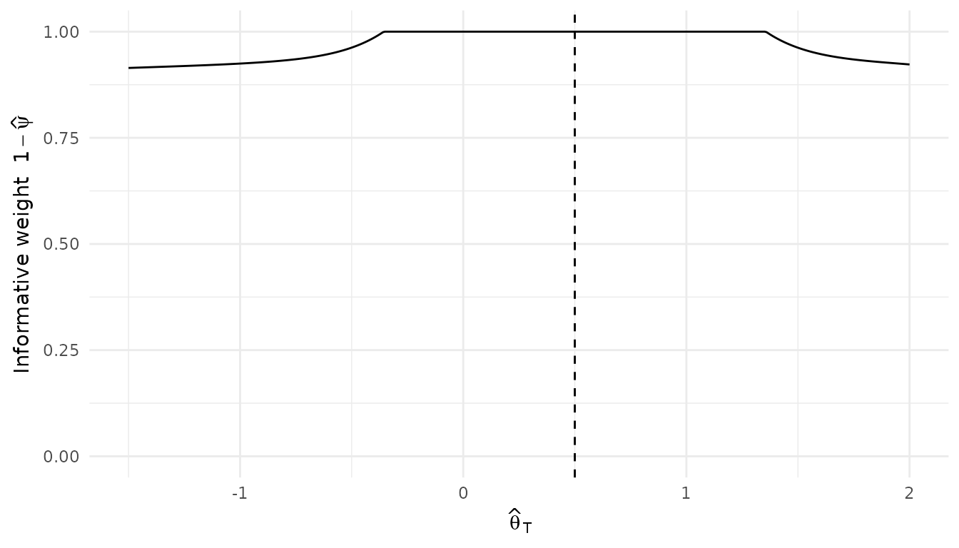

The dashed line marks the source estimate. Note that the curve is not symmetric about it: the weak component is centred at $\theta_0 = 0$ rather than at the source estimate, so an estimate falling short of the source is easier for the weak component to explain than one overshooting it by the same amount.

The binary endpoint

For the Aprepitant case study the target statistic is the pair of responder counts $(y_c, y_t)$, and the analysis model is the binomial RMP’s. Its informative component is the source posterior of the rate difference carried to the target, i.e. the conditional power prior with full borrowing; its weak component gives both target response rates independent uniform priors. Both are observed through two binomial arms.

The sample space is finite, so the conflict $p$-value is computed exactly by enumeration rather than by substituting a different statistic. For each component

$$m_j(y_c, y_t) = \int p(y_c, y_t \mid \theta_T, p_c)\, j(\theta_T, p_c)\, d\theta_T\, dp_c,$$

which is tabulated over $y_c = 0, \ldots, N_T^{(c)}$ and $y_t = 0, \ldots, N_T^{(t)}$. Under the weak component every pair of counts is equally likely, so its table is exactly uniform. Then

$$P_\psi(y_c^{\mathrm{obs}}, y_t^{\mathrm{obs}}) = \sum_{\{(y_c, y_t)\, :\, m_\psi(y_c, y_t) \le m_\psi(y_c^{\mathrm{obs}}, y_t^{\mathrm{obs}})\}} m_\psi(y_c, y_t).$$

source_counts <- list(
  n_control_source = 280L, n_successes_control_source = 154L,
  n_treatment_source = 293L, n_successes_treatment_source = 184L
)
components <- BExTE:::binomial_rmp_components(source_counts)
tables <- BExTE:::binomial_rmp_predictive_tables(
  components, source_counts, n_control = 52, n_treatment = 55
)
informative_table <- tables$informative
weak_table <- tables$weak

# The tables enumerate the whole sample space, so they sum to one.
c(informative = sum(informative_table), weak = sum(weak_table))

## informative        weak 
##           1           1

BExTE:::egidi_select_weak_weight_binomial(
  table_informative = informative_table,
  table_weak = weak_table,
  y_control = 42, y_treatment = 48,
  alpha_pc = 0.05
)

##   psi_weak pvalue_informative pvalue_weak pvalue_selected initial_conflict
## 1        0          0.7417261           1       0.7417261            FALSE
##   conflict_unresolved
## 1               FALSE

Configuration

The method is registered as egidi_empirical_mixture. It has no weight to sweep, so it contributes a single parameter combination:

egidi_empirical_mixture:
  alpha_pc: 0.05
  pvalue_method: exact
  weight_grid_step: 0.001
  empirical_bayes: TRUE

alpha_pc is 0.05 in the primary analysis; 0.01 and 0.10 are the sensitivity values.