Introduction
This vignette describes an implementation of a Bayesian analysis that pools the source and target study data.
Posterior distribution
With pooling, the prior distribution of is given by:
We observe data points with sample mean and known variance . This implies the likelihood is given by:
Since both the prior and the likelihood are Gaussian distributions, the posterior will also be a Gaussian distribution.
The posterior distribution is :
Posterior Mean:
Posterior Variance:
Thus, the posterior distribution is:
In the limit where goes to infinity:
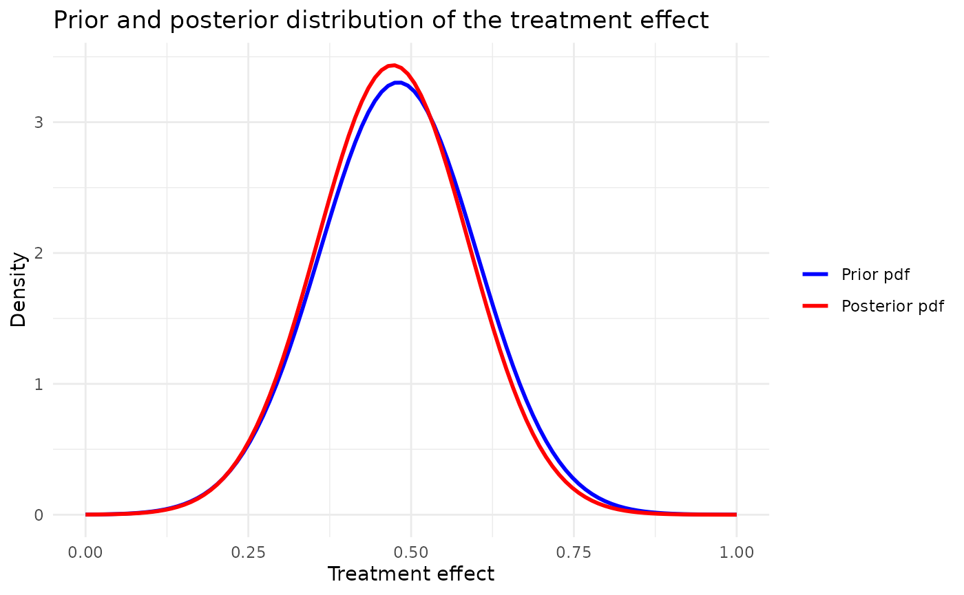
That is, the target study data are discarded because the likelihood becomes flat, and the posterior is the same as the prior.
Pooling the data is equivalent to defining a Gaussian prior with mean and standard deviation corresponding to the treatment effect estimate and standard error on the treatment effect in the source study.
Load the case study configuration
Load the simulation configuration and the Belimumab case study configuration from YAML files.
set.seed(42)
case_study_config <- yaml::yaml.load_file(system.file("conf/case_studies/belimumab.yml", package = "BExTE"))
Create data objects
Create a source_data instance, where information about the source data is stored
source_data <- ObservedSourceData$new(case_study_config)Set the observed target data (in the paediatrics population)
target_data <- ObservedTargetData$new(treatment_effect_estimate = case_study_config$target$treatment_effect, treatment_effect_standard_error = case_study_config$target$standard_error, target_sample_size_per_arm = as.integer(case_study_config$target$total / 2), summary_measure_likelihood = case_study_config$summary_measure_likelihood)Create model
method <- "pooling"
method_parameters <- list(
  initial_prior = "noninformative" # This corresponds to the fact that the posterior for the adults data is derived from an uninformative prior (for consistency with other methods).
)
Now, we define the model we want to use for inferring the treatment effect in the target study.
model <- Model$new()

model <- model$create(
  case_study_config = case_study_config,
  method = method,
  method_parameters = method_parameters,
  source_data = source_data
)
This model calls RBesT in the backend, leveraging the fact that it is a special case of a Robust Mixture Prior.