Load the case study configuration
Load the simulation configuration and the Belimumab case study configuration from YAML files.
set.seed(42)
simulation_config <- yaml::yaml.load_file(system.file("conf/simulation_config.yml", package = "BExTE"))

case_study <- "belimumab"
case_study_config <- yaml::yaml.load_file(system.file("conf/case_studies/belimumab.yml", package = "BExTE"))
Method and scenario
Create a source_data instance, where information about the source data is stored
source_data <- SourceData$new(case_study_config)

target_sample_size_per_arm <- as.integer(case_study_config$source$total / 2)
method <- "pooling"
method_parameters <- list(
  initial_prior = "noninformative", # This corresponds to the fact that the posterior for the adults data is derived from an uninformative prior (for consistency with other methods).
  empirical_bayes = FALSE # Corresponds to whether some parameters of the prior are based on observed data.
)
Now, we define the model we want to use for inferring the treatment effect in the target study.
model <- Model$new()

model <- model$create(
  case_study_config = case_study_config,
  method = method,
  method_parameters = method_parameters,
  source_data = source_data
)
Simulation
Separate analysis:
separate_method <- "separate"
method_parameters <- list(
  initial_prior = "noninformative", # This corresponds to the fact that the posterior for the adults data is derived from an uninformative prior (for consistency with other methods).
  empirical_bayes = FALSE # Corresponds to whether some parameters of the prior are based on observed data.
)

separate_model <- Model$new()

separate_model <- separate_model$create(
  case_study_config = case_study_config,
  method = separate_method,
  method_parameters = method_parameters,
  source_data = source_data
)
treatment_effect_values <- seq(-7, 2, length.out = 200)

n <- length(treatment_effect_values)
confidence_level <- simulation_config$confidence_level
null_space <- case_study_config$null_space

n_replicates <- 100

separate_test_decisions <- matrix(rep(0, n * n_replicates), nrow = n)
separate_posterior_means <- matrix(rep(0, n * n_replicates), nrow = n)
separate_posterior_medians <- matrix(rep(0, n * n_replicates), nrow = n)
separate_credible_intervals <- array(rep(0, n * n_replicates * 2), dim = c(n, n_replicates, 2))
separate_prior_proba_no_benefit <- rep(0, n)

theta_0 <- case_study_config$theta_0

critical_value <- simulation_config$critical_value


for (i in seq_along(treatment_effect_values)) {
  drift <- treatment_effect_values[i] - source_data$treatment_effect_estimate
  target_data <- TargetDataFactory$new()

  target_data <- target_data$create(source_data = source_data, case_study_config = case_study_config, target_sample_size_per_arm = target_sample_size_per_arm, treatment_drift = drift, summary_measure_likelihood = source_data$summary_measure_likelihood)

  results <- separate_model$simulation_for_given_treatment_effect(target_data = target_data, n_replicates = n_replicates, critical_value = critical_value, theta_0 = theta_0, confidence_level = confidence_level, null_space = null_space, to_return = c("test_decision", "posterior_mean", "posterior_median", "credible_interval"),  method = method, case_study = case_study, n_samples_quantiles_estimation = simulation_config$n_samples_quantiles_estimation)

  separate_test_decisions[i, ] <- results$test_decisions
  separate_posterior_means[i, ] <- results$posterior_means
  separate_posterior_medians[i, ] <- results$posterior_medians
  separate_credible_intervals[i, , ] <- matrix(results$credible_intervals, nrow = n_replicates)
}
test_decisions <- matrix(rep(0, n * n_replicates), nrow = n)
posterior_means <- matrix(rep(0, n * n_replicates), nrow = n)
posterior_medians <- matrix(rep(0, n * n_replicates), nrow = n)
credible_intervals <- array(rep(0, n * n_replicates * 2), dim = c(n, n_replicates, 2))
prior_proba_no_benefit <- rep(0, n)

for (i in seq_along(treatment_effect_values)) {
  drift <- treatment_effect_values[i] - source_data$treatment_effect_estimate # This implies that target_data$treatment_effect <- treatment_effect_values[i]
  target_data <- TargetDataFactory$new()

  target_data <- target_data$create(source_data = source_data, case_study_config = case_study_config, target_sample_size_per_arm = target_sample_size_per_arm, treatment_drift = drift, summary_measure_likelihood = source_data$summary_measure_likelihood)

  # target_data$sampling_approximation <- TRUE
  results <- model$simulation_for_given_treatment_effect(target_data = target_data, n_replicates = n_replicates, critical_value = critical_value, theta_0 = theta_0, confidence_level = confidence_level, null_space = null_space, to_return = c("test_decision", "posterior_mean", "posterior_median", "credible_interval"),  method = method, case_study = case_study, n_samples_quantiles_estimation = simulation_config$n_samples_quantiles_estimation)

  test_decisions[i, ] <- results$test_decisions
  posterior_means[i, ] <- results$posterior_means
  posterior_medians[i, ] <- results$posterior_medians
  credible_intervals[i, , ] <- matrix(results$credible_intervals, nrow = n_replicates)
}
conditional_proba_success <- rowMeans(test_decisions) # Contains Pr(Study success | theta_T)
data <- data.frame(conditional_proba_success = conditional_proba_success, treatment_effect_values = treatment_effect_values, method = method)

separate_conditional_proba_success <- rowMeans(separate_test_decisions) # Contains Pr(Study success | theta_T)

separate_data <- data.frame(conditional_proba_success = separate_conditional_proba_success, treatment_effect_values = treatment_effect_values, method = separate_method)

combined_data <- rbind(data, separate_data)

plt <- ggplot(combined_data, aes(x = treatment_effect_values, y = conditional_proba_success, color = method)) +
  geom_point() +
  ggplot2::labs(
    title = "Posterior mean vs Target Treatment Effect",
    x = "Target Treatment Effect",
    y = "Success probability",
    color = "Method"
  ) +
  theme_minimal()

print(plt)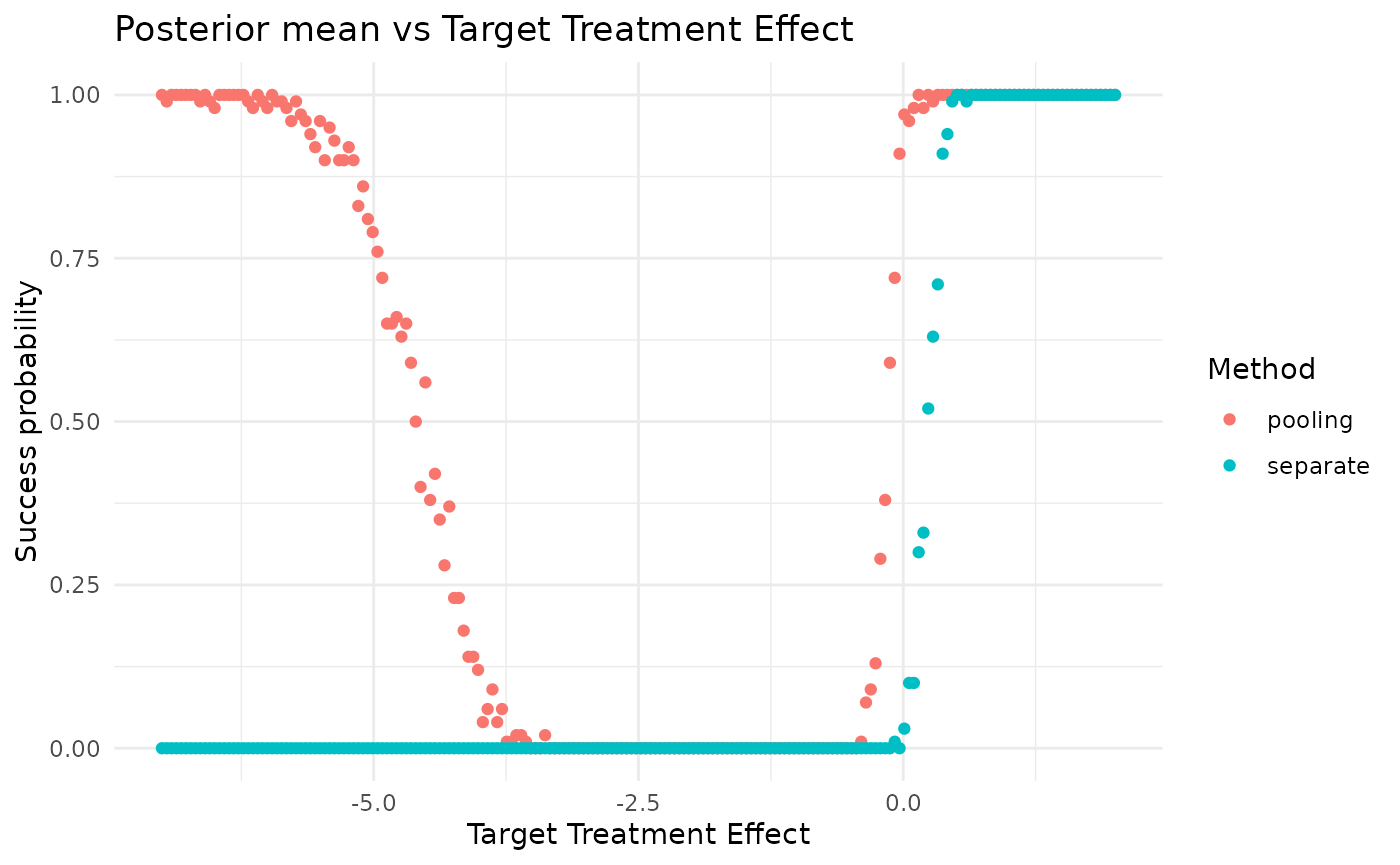
separate_conditional_posterior_means <- rowMeans(separate_posterior_means)
separate_data <- data.frame(conditional_posterior_means = separate_conditional_posterior_means, treatment_effect_values = treatment_effect_values, method = separate_method)

conditional_posterior_means <- rowMeans(posterior_means)
data <- data.frame(conditional_posterior_means = conditional_posterior_means, treatment_effect_values = treatment_effect_values, method = method)

combined_data <- rbind(data, separate_data)

plt <- ggplot(combined_data, aes(x = treatment_effect_values, y = conditional_posterior_means, color = method)) +
  geom_point() +
  ggplot2::labs(
    title = "Posterior mean vs Target Treatment Effect",
    x = "Target Treatment Effect",
    y = "Posterior mean",
    color = "Method"
  ) +
  theme_minimal()

print(plt)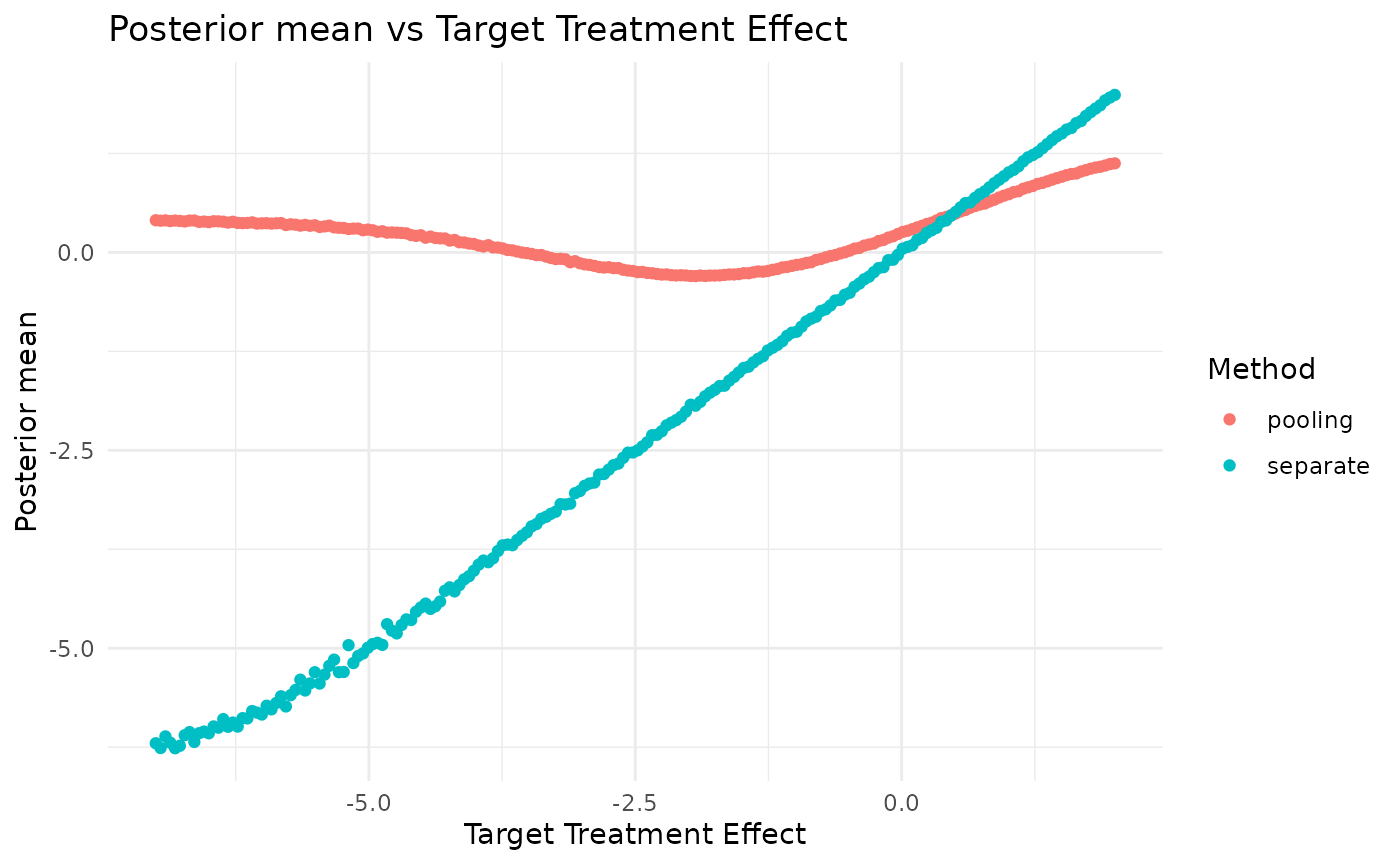
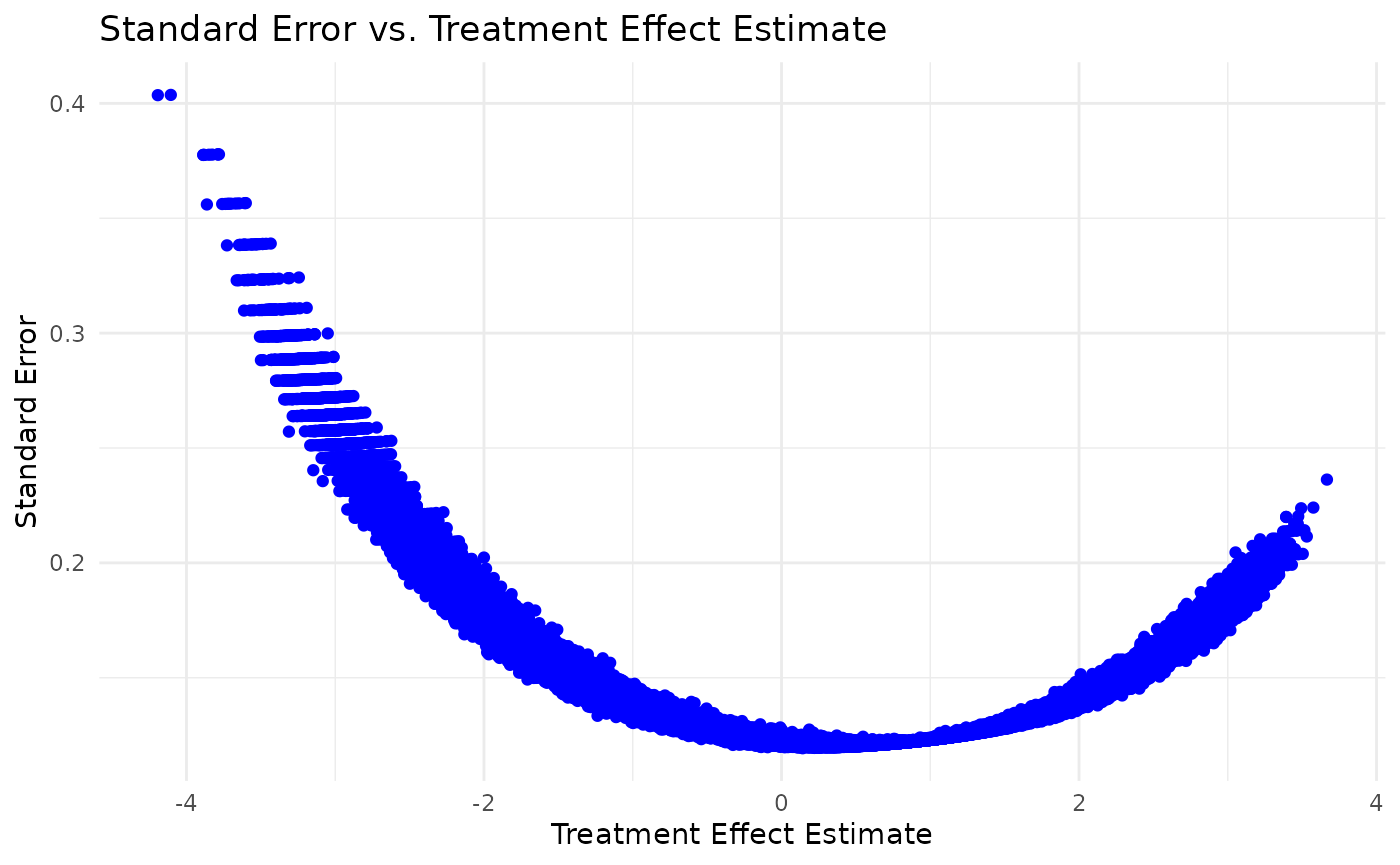
Standard error vs treatment effect estimate
# Define a vector of treatment effect values to loop over
treatment_effect_values <- seq(-3, 3, by = 0.1)

# Initialize an empty list to store dataframes
data_list <- list()

# Loop over treatment effect values
for (treatment_effect in treatment_effect_values) {
  # Calculate the drift
  drift <- treatment_effect - source_data$treatment_effect_estimate

  # Create target data
  target_data <- TargetDataFactory$new()
  target_data <- target_data$create(
    source_data = source_data,
    case_study_config = case_study_config,
    target_sample_size_per_arm = target_sample_size_per_arm,
    treatment_drift = drift,
    summary_measure_likelihood = source_data$summary_measure_likelihood
  )

  # Generate samples
  samples <- target_data$generate(1000)

  # Create a dataframe from the samples
  data <- data.frame(
    treatment_effect = treatment_effect,
    treatment_effect_estimate = samples$treatment_effect_estimate,
    treatment_effect_standard_error = samples$treatment_effect_standard_error
  )

  # Append the dataframe to the list
  data_list[[length(data_list) + 1]] <- data
}

# Combine all dataframes into a single dataframe
combined_data <- dplyr::bind_rows(data_list)

ggplot(combined_data, aes(x = treatment_effect_estimate, y = treatment_effect_standard_error)) +
  geom_point(color = "blue") +
  ggplot2::labs(
    title = "Standard Error vs. Treatment Effect Estimate",
    x = "Treatment Effect Estimate",
    y = "Standard Error"
  ) +
  theme_minimal()