Replication of the Belimumab case study

Introduction

This code replicates the analysis presented in Best et al (2023), initially reported in Pottackal et al (2019).

Set working directory, import functions and configurations

Load the Belimumab case study configuration from YAML files.

set.seed(42)

case_study_config <- yaml::yaml.load_file(system.file("conf/case_studies/belimumab.yml", package = "BExTE"))

Define the method used (RMP) and the range of parameters considered

Define the range of values considered for the weight on the informative component of the RMP

method <- "RMP"
Nw <- 21
w_range <- seq(0, 1, length.out = Nw)

Define the method’s parameters

method_parameters <- list(
  initial_prior = "noninformative", # This corresponds to the fact that the posterior for the adults data is derived from an uninformative prior (for consistency with other methods). May be removed in future releases.
  prior_weight = 0.5, # weight on the informative component of the mixture
  empirical_bayes = TRUE
)

Create data objects

Create a source_data instance, where information about the source data is stored

source_data <- ObservedSourceData$new(case_study_config)

Set the observed target data (in the paediatric population)

target_data <- ObservedTargetData$new(treatment_effect_estimate = case_study_config$target$treatment_effect, treatment_effect_standard_error = case_study_config$target$standard_error, target_sample_size_per_arm = as.integer(case_study_config$target$total / 2), summary_measure_likelihood = case_study_config$summary_measure_likelihood)

Note that, at the moment, the code does not allow specifying different sample sizes for the arms of the target study.

Inference

For each parameter, instantiate a model, perform Bayesian inference and compute the posterior mean and credible interval.

point_est <- numeric(Nw)
credible_intervals <- matrix(NA, 2, Nw)
confidence_level <- 0.95
lower_quantile <- (1 - confidence_level) / 2
upper_quantile <- 1 - lower_quantile

posterior_w <- numeric(Nw)

The model instantiation relies on the so-called factory design pattern for increased ease of use and flexibility.

for (i in seq_along(w_range)) {
  method_parameters$prior_weight <- w_range[i]

  model <- Model$new()
  model <- model$create(
    case_study_config = case_study_config,
    method = method,
    method_parameters = method_parameters,
    source_data = source_data
  )

  # Perform Bayesian inference based on observed target data.
  model$inference(target_data = target_data)

  # Convert the estimates back to the natural scale
  point_est[i] <- exp(model$posterior_mean())

  # To estimate the credible intervals, we sample from the posterior distribution
  posterior_samples <- exp(model$sample_posterior(10000))
  credible_intervals[, i] <- quantile(posterior_samples, probs = c(lower_quantile, upper_quantile))
  posterior_w[i] <- model$wpost
}

Plot the results

We plot the results as in the original paper by Pottackal et al (2019).

ggplot2::ggplot() +
  geom_errorbar(ggplot2::aes(x = w_range, y = point_est, ymin = credible_intervals[1, ], ymax = credible_intervals[2, ]),
    color = "black", linewidth = 1, width = 0
  ) +
  geom_point(ggplot2::aes(x = w_range, y = point_est), color = "black") +
  geom_hline(yintercept = 1, linetype = "dashed", linewidth = 1) +
  ggplot2::labs(
    x = "Prior weight on adult data",
    y = "Odds ratio (95% CrI, log scale)",
    title = "Posterior Mean with the Gaussian RMP"
  ) +
  scale_y_log10(breaks = c(0.7, 0.9, 1, 1.5, 2, 3)) +
  theme_minimal() +
  theme(plot.title = element_text(hjust = 0.5))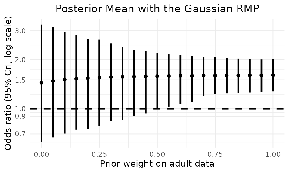

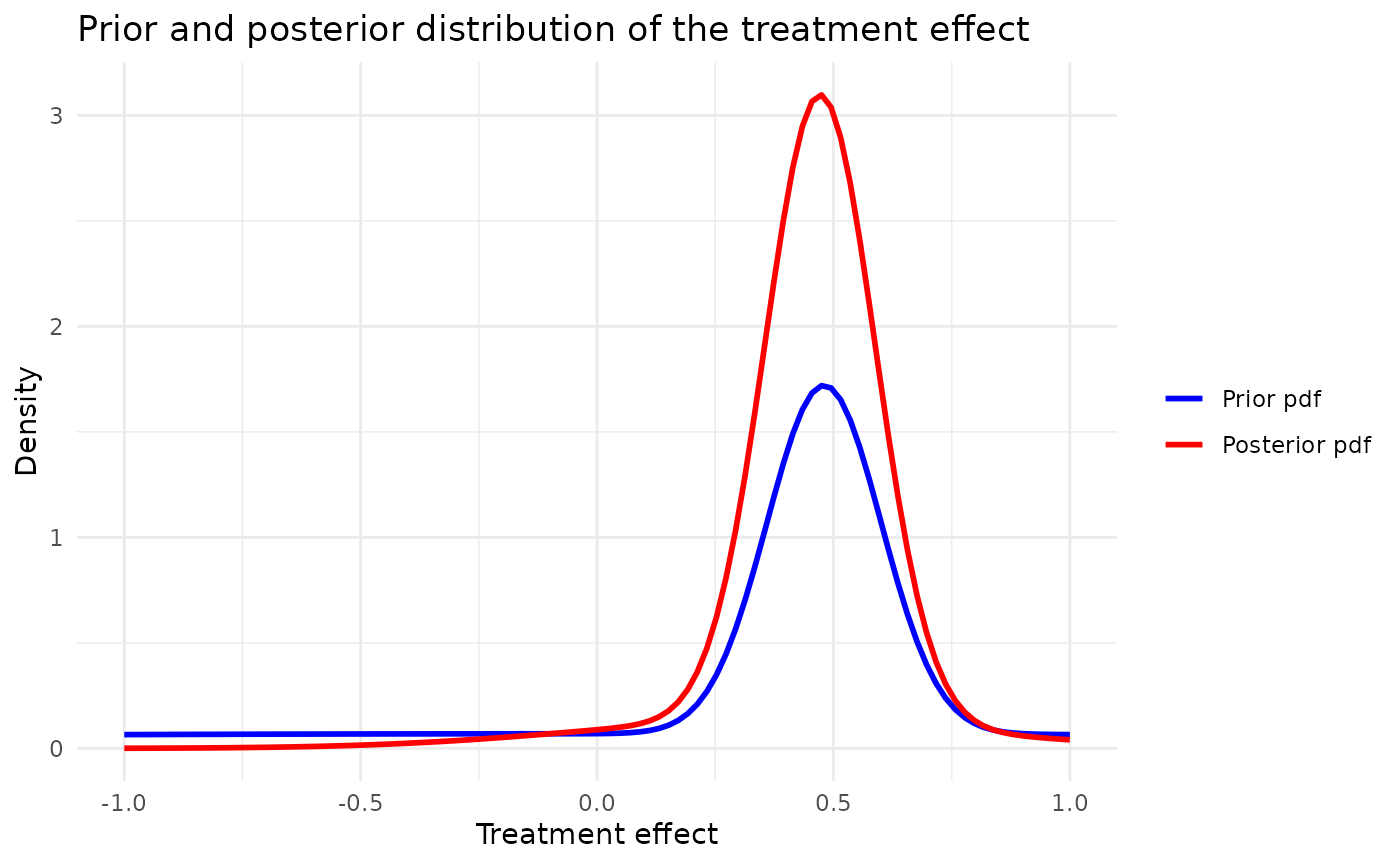
Posterior and prior pdf :

method_parameters$prior_weight <- 0.5

model <- Model$new()
model <- model$create(
  case_study_config = case_study_config,
  method = method,
  method_parameters = method_parameters,
  source_data = source_data
)

# Perform Bayesian inference based on observed target data.
model$inference(target_data = target_data)

## [1] "Success"