Replication of the Mepolizumab case study

Introduction

This code replicates the analysis presented in Best et al (2021).

Set working directory, import functions and configurations

Load the Mepolizumab case study configuration from YAML files.

set.seed(42)
config_path <- system.file("conf/case_studies/mepolizumab.yml", package = "BExTE")
case_study_config <- yaml::yaml.load_file(config_path)

Define the method used (RMP) and the range of parameters considered

Define the range of values considered for the weight on the informative component of the RMP

method <- "RMP"
Nw <- 20
w_range <- seq(0, 1, length.out = Nw)

Define the method’s parameters

method_parameters <- list(
  initial_prior = "noninformative", # This corresponds to the fact that the posterior for the adults data is derived from an uninformative prior (for consistency with other methods). May be removed in future releases.
  prior_weight = 0.5, # weight on the informative component of the mixture
  empirical_bayes = FALSE
)

Set the vague component variance using the target data variance (as in Best et al (2021) for Mepolizumab). The vague prior corresponds to the information provided by a single subject.

vague_prior_variance <- case_study_config$target$standard_error^2 * case_study_config$target$total
# This is obtained by setting
empirical_bayes <- TRUE

Create data objects

Create a source_data instance, where information about the source data is stored

source_data <- ObservedSourceData$new(case_study_config)

Set the observed target data (in the paediatrics population)

target_data <- ObservedTargetData$new(treatment_effect_estimate = case_study_config$target$treatment_effect, treatment_effect_standard_error = case_study_config$target$standard_error, target_sample_size_per_arm = as.integer(case_study_config$target$total / 2), summary_measure_likelihood = case_study_config$summary_measure_likelihood)

print(target_data$sample)

## $treatment_effect_estimate
## [1] -0.395
## 
## $treatment_effect_standard_error
## [1] 0.703

n_paediatrics <- as.integer(case_study_config$target$total / 2)

$\text { Robust mixture prior } =w \times \operatorname{Normal}\left(m_{\text {adult }}, v_{\text {adult }}\right)+(1-w) \times \operatorname{Normal}\left(m_{\text {weak }}, v_{\text {weak }}\right)$

$\text { Robust mixture prior }=w \times \operatorname{Normal}(-0.694,0.017)+(1-w) \times \operatorname{Normal}(0,12.4)$

Note that, at the moment, the code does not allow specifying different sample sizes for the arms of the target study.

Inference

For each parameter, instantiate a model, perform Bayesian inference and compute the posterior mean and credible interval.

The model instantiation relies on the so-called factory design pattern for increased ease of use and flexibility.

n_samples_posterior <- 10000000

point_est <- numeric(Nw)
credible_intervals <- matrix(NA, 2, Nw)
confidence_level <- 0.95
lower_quantile <- (1 - confidence_level) / 2
upper_quantile <- 1 - lower_quantile

posterior_w <- numeric(Nw)

for (i in seq_along(w_range)) {
  method_parameters$prior_weight <- w_range[i]

  model <- Model$new()
  model <- model$create(
    case_study_config = case_study_config,
    method = method,
    method_parameters = method_parameters,
    source_data = source_data
  )

  model$vague_prior_variance <- n_paediatrics * target_data$sample$treatment_effect_standard_error^2 # Following Best et al, 2021.

  # Perform Bayesian inference based on observed target data.
  model$inference(target_data = target_data)

  # Convert the estimates back to the natural scale
  point_est[i] <- exp(model$posterior_mean())

  # To estimate the credible intervals, we sample from the posterior distribution
  posterior_samples <- exp(model$sample_posterior(n_samples_posterior))
  credible_intervals[, i] <- quantile(posterior_samples, probs = c(lower_quantile, upper_quantile))
  posterior_w[i] <- model$wpost
}

Plot results

We plot the results as in the original paper by Best et al (2021).

ggplot2::ggplot() +
  geom_errorbar(
    ggplot2::aes(
      x = w_range,
      y = point_est,
      ymin = credible_intervals[1, ],
      ymax = credible_intervals[2, ]
    ),
    color = "black", linewidth = 1, width = 0
  ) +
  geom_point(ggplot2::aes(x = w_range, y = point_est), color = "black", size = 3) +
  geom_hline(yintercept = 1, linetype = "dashed", linewidth = 1) +
  ggplot2::labs(
    x = "Prior weight on adult data",
    y = "Rates ratio (95% CI, log scale)",
    title = "Posterior Mean with the Gaussian RMP"
  ) +
  scale_y_log10(limits = c(0.0625, 4), breaks = c(0.0625, 0.125, 0.25, 0.5, 1, 2, 4)) +
  theme_bw() +
  theme(
    text = element_text(size = 14),
    axis.text.y = element_text(size = 7),
    axis.ticks.y = element_blank(),
    strip.text.x = element_text(size = 10),
    legend.key = element_blank(),
    strip.background = element_blank(),
    panel.grid.major = element_blank(),
    panel.grid.minor = element_blank()
  )

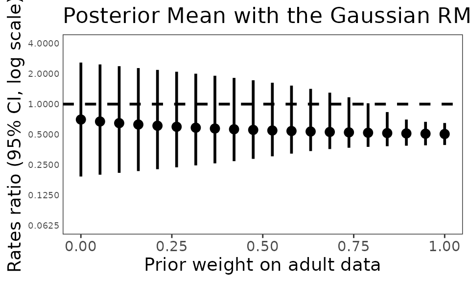
Table summarizing the results

Best et al (2021) presents a table summarizing the results of inference for various prior weights.

data <- data.frame(
  "Prior weight on adult data" = seq(0, 1, by = 0.1),
  "Rate Ratio (95% CrI) (Mepo/Placebo)" = c(
    "0.68 (0.18, 2.64)",
    "0.55 (0.20, 2.33)",
    "0.53 (0.23, 2.07)",
    "0.52 (0.25, 1.85)",
    "0.51 (0.28, 1.64)",
    "0.51 (0.32, 1.44)",
    "0.51 (0.36, 1.23)",
    "0.51 (0.37, 0.99)",
    "0.51 (0.38, 0.74)",
    "0.51 (0.39, 0.67)",
    "0.50 (0.39, 0.65)"
  ),
  check.names = FALSE
)

# Create and style the table
kable(data, "html") %>%
  kableExtra::kable_styling("striped", full_width = F)

Prior weight on adult data	Rate Ratio (95% CrI) (Mepo/Placebo)
0.0	0.68 (0.18, 2.64)
0.1	0.55 (0.20, 2.33)
0.2	0.53 (0.23, 2.07)
0.3	0.52 (0.25, 1.85)
0.4	0.51 (0.28, 1.64)
0.5	0.51 (0.32, 1.44)
0.6	0.51 (0.36, 1.23)
0.7	0.51 (0.37, 0.99)
0.8	0.51 (0.38, 0.74)
0.9	0.51 (0.39, 0.67)
1.0	0.50 (0.39, 0.65)

Nw <- 11
w_range <- seq(0, 1, length.out = Nw)
point_est <- numeric(Nw)
credible_intervals <- matrix(NA, 2, Nw)
confidence_level <- 0.95
lower_quantile <- (1 - confidence_level) / 2
upper_quantile <- 1 - lower_quantile

posterior_w <- numeric(Nw)

for (i in seq_along(w_range)) {
  method_parameters$prior_weight <- w_range[i]

  model <- Model$new()
  model <- model$create(
    case_study_config = case_study_config,
    method = method,
    method_parameters = method_parameters,
    source_data = source_data
  )
  model$vague_prior_variance <- n_paediatrics * target_data$sample$treatment_effect_standard_error^2 # Following Best et al, 2021.

  # Perform Bayesian inference based on observed target data.
  model$inference(target_data = target_data)

  # Convert the estimates back to the natural scale
  point_est[i] <- exp(model$posterior_mean())

  # To estimate the credible intervals, we sample from the posterior distribution
  posterior_samples <- exp(model$sample_posterior(n_samples_posterior))
  credible_intervals[, i] <- quantile(posterior_samples, probs = c(lower_quantile, upper_quantile))
  posterior_w[i] <- model$wpost
}


point_est <- round(point_est, 2)
credible_intervals <- round(credible_intervals, 2)

data <- data.frame(
  `Prior weight on adult data` = w_range,
  `Rate Ratio (95% CrI) (Mepo/Placebo)` = paste(
    point_est,
    paste0("(", round(credible_intervals[1, ], 2), ", ", round(credible_intervals[2, ], 2), ")")
  ),
  check.names = FALSE
)
# Create and style the table
kable(data, "html", escape = FALSE) %>%
  kableExtra::kable_styling("striped", full_width = F)

Prior weight on adult data	Rate Ratio (95% CrI) (Mepo/Placebo)
0.0	0.7 (0.19, 2.58)
0.1	0.65 (0.21, 2.39)
0.2	0.61 (0.22, 2.2)
0.3	0.59 (0.24, 2.03)
0.4	0.57 (0.27, 1.86)
0.5	0.55 (0.29, 1.68)
0.6	0.54 (0.33, 1.48)
0.7	0.53 (0.36, 1.26)
0.8	0.52 (0.38, 0.99)
0.9	0.51 (0.39, 0.7)
1.0	0.5 (0.39, 0.65)

Posterior weight vs prior weight

Best et al (2021) contains a figure representing the posterior weight on adult data as a function of the prior weight on adult data.

data <- data.frame(
  w = w_range,
  posterior_w = posterior_w
)

scatter_plot <- ggplot2::ggplot(data, ggplot2::aes(x = w_range, y = posterior_w)) +
  geom_point() +
  ggtitle("Prior versus posterior weight on adult component of the robust mixture prior") +
  xlab("Prior weight on adult data") +
  ylab("Posterior weight on adult data") +
  theme_minimal() +
  theme(plot.title = element_text(hjust = 0.5))

print(scatter_plot)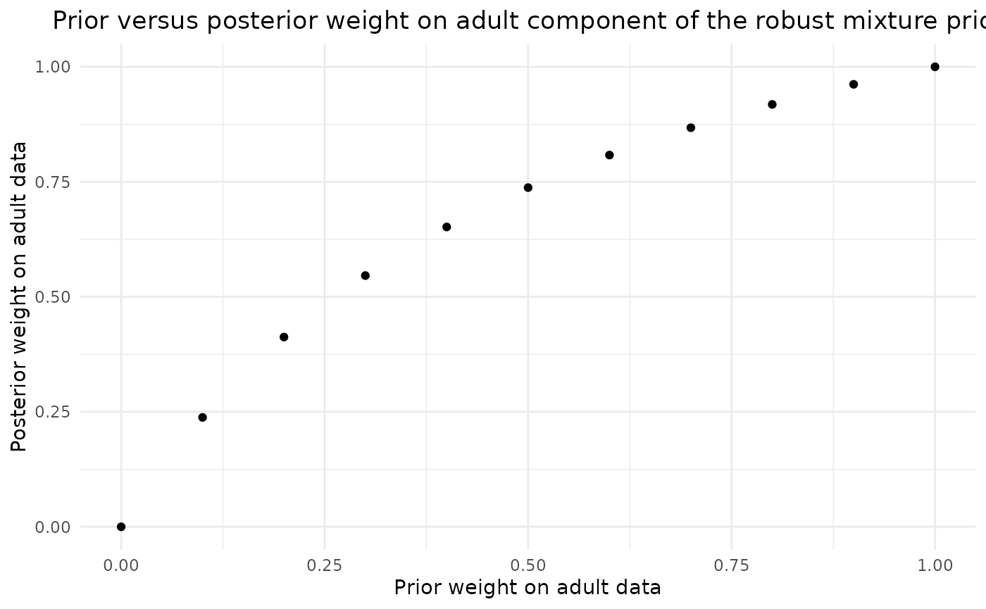

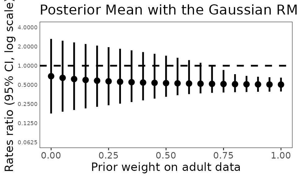
Comparison with RBesT

Nw <- 21
w_range <- seq(0, 1, length.out = Nw)
point_est <- numeric(Nw)
credible_intervals <- matrix(NA, 2, Nw)
confidence_level <- 0.95
lower_quantile <- (1 - confidence_level) / 2
upper_quantile <- 1 - lower_quantile

posterior_w <- numeric(Nw)

for (i in seq_along(w_range)) {
  prior.sri <- RBesT::mixnorm(c(w_range[i], source_data$treatment_effect_estimate, sqrt(0.017)), c(1 - w_range[i], 0, sqrt(12.4)))
  post.sri <- RBesT::postmix(prior.sri, m = target_data$sample$treatment_effect_estimate, se = target_data$sample$treatment_effect_standard_error)
  res.sri <- summary(post.sri)

  # Convert the estimates back to the natural scale
  point_est[i] <- exp(res.sri["mean"])

  credible_intervals[, i] <- c(exp(res.sri[3]), exp(res.sri[5]))
}

ggplot2::ggplot() +
  geom_errorbar(
    ggplot2::aes(
      x = w_range,
      y = point_est,
      ymin = credible_intervals[1, ],
      ymax = credible_intervals[2, ]
    ),
    color = "black", linewidth = 1, width = 0
  ) +
  geom_point(ggplot2::aes(x = w_range, y = point_est), color = "black", size = 3) +
  geom_hline(yintercept = 1, linetype = "dashed", linewidth = 1) +
  ggplot2::labs(
    x = "Prior weight on adult data",
    y = "Rates ratio (95% CI, log scale)",
    title = "Posterior Mean with the Gaussian RMP"
  ) +
  scale_y_log10(limits = c(0.0625, 4), breaks = c(0.0625, 0.125, 0.25, 0.5, 1, 2, 4)) +
  theme_bw() +
  theme(
    text = element_text(size = 14),
    axis.text.y = element_text(size = 7),
    axis.ticks.y = element_blank(),
    strip.text.x = element_text(size = 10),
    legend.key = element_blank(),
    strip.background = element_blank(),
    panel.grid.major = element_blank(),
    panel.grid.minor = element_blank()
  )

Nw <- 11
w_range <- seq(0, 1, length.out = Nw)
point_est <- numeric(Nw)
credible_intervals <- matrix(NA, 2, Nw)
confidence_level <- 0.95
lower_quantile <- (1 - confidence_level) / 2
upper_quantile <- 1 - lower_quantile

posterior_w <- numeric(Nw)

for (i in seq_along(w_range)) {
  prior.sri <- RBesT::mixnorm(c(w_range[i], source_data$treatment_effect_estimate, sqrt(0.017)), c(1 - w_range[i], 0, sqrt(12.4)))
  post.sri <- RBesT::postmix(prior.sri, m = target_data$sample$treatment_effect_estimate, se = target_data$sample$treatment_effect_standard_error)
  res.sri <- summary(post.sri)


  model$vague_prior_variance <- n_paediatrics * target_data$sample$treatment_effect_standard_error^2 # Following Best et al, 2021.

  # Perform Bayesian inference based on observed target data.
  model$inference(target_data = target_data)

  # Convert the estimates back to the natural scale
  point_est[i] <- exp(res.sri["mean"])

  # To estimate the credible intervals, we sample from the posterior distribution
  posterior_samples <- exp(RBesT::rmix(post.sri, n = n_samples_posterior))
  credible_intervals[, i] <- quantile(posterior_samples, probs = c(lower_quantile, upper_quantile))
}

point_est <- round(point_est, 2)
credible_intervals <- round(credible_intervals, 2)

data <- data.frame(
  `Prior weight on adult data` = w_range,
  `Rate Ratio (95% CrI) (Mepo/Placebo)` = paste(
    point_est,
    paste0("(", round(credible_intervals[1, ], 2), ", ", round(credible_intervals[2, ], 2), ")")
  ),
  check.names = FALSE
)
# Create and style the table
kable(data, "html", escape = FALSE) %>%
  kableExtra::kable_styling("striped", full_width = F)

Prior weight on adult data	Rate Ratio (95% CrI) (Mepo/Placebo)
0.0	0.68 (0.18, 2.64)
0.1	0.62 (0.2, 2.33)
0.2	0.58 (0.23, 2.07)
0.3	0.56 (0.25, 1.85)
0.4	0.54 (0.29, 1.64)
0.5	0.53 (0.32, 1.44)
0.6	0.52 (0.36, 1.23)
0.7	0.52 (0.37, 0.99)
0.8	0.51 (0.38, 0.74)
0.9	0.51 (0.39, 0.67)
1.0	0.5 (0.39, 0.65)

Other treatment effect values in the target study

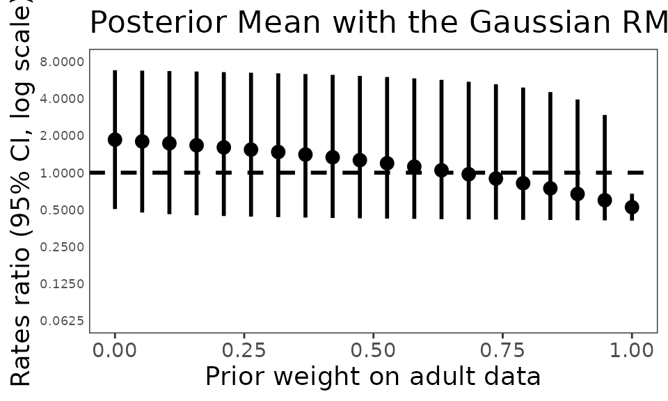
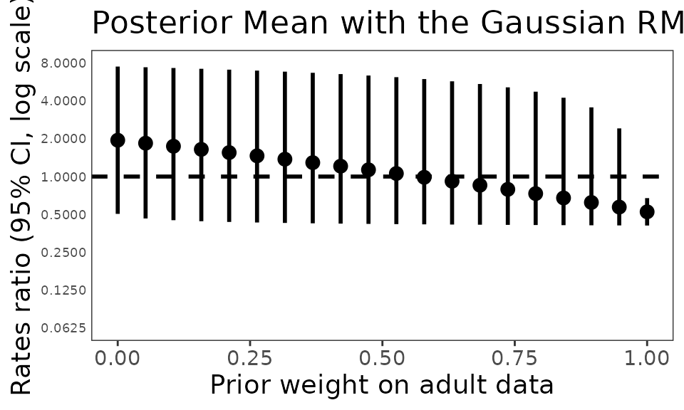
In Figure 5 of Best et al (2021), several other values are considered for the RR in adolescents (2, 1.25, 0.9, 0.3):

target_data$sample$treatment_effect_estimate <- log(2)


Nw <- 20
point_est <- numeric(Nw)
w_range <- seq(0, 1, length.out = Nw)
credible_intervals <- matrix(NA, 2, Nw)

posterior_w <- numeric(Nw)

for (i in seq_along(w_range)) {
  method_parameters$prior_weight <- w_range[i]

  model <- Model$new()
  model <- model$create(
    case_study_config = case_study_config,
    method = method,
    method_parameters = method_parameters,
    source_data = source_data
  )

  model$vague_prior_variance <- n_paediatrics * target_data$sample$treatment_effect_standard_error^2 # Following Best et al, 2021.

  # Perform Bayesian inference based on observed target data.
  model$inference(target_data = target_data)

  # Convert the estimates back to the natural scale
  point_est[i] <- exp(model$posterior_mean())

  # To estimate the credible intervals, we sample from the posterior distribution
  posterior_samples <- exp(model$sample_posterior(n_samples_posterior))
  credible_intervals[, i] <- quantile(posterior_samples, probs = c(lower_quantile, upper_quantile))
  posterior_w[i] <- model$wpost
}

Plot results

We plot the results as in the original paper by Best et al (2021)

ggplot2::ggplot() +
  geom_errorbar(
    ggplot2::aes(
      x = w_range,
      y = point_est,
      ymin = credible_intervals[1, ],
      ymax = credible_intervals[2, ]
    ),
    color = "black", linewidth = 1, width = 0
  ) +
  geom_point(ggplot2::aes(x = w_range, y = point_est), color = "black", size = 3) +
  geom_hline(yintercept = 1, linetype = "dashed", linewidth = 1) +
  ggplot2::labs(
    x = "Prior weight on adult data",
    y = "Rates ratio (95% CI, log scale)",
    title = "Posterior Mean with the Gaussian RMP"
  ) +
  scale_y_log10(limits = c(0.0625, 8), breaks = c(0.0625, 0.125, 0.25, 0.5, 1, 2, 4, 8)) +
  theme_bw() +
  theme(
    text = element_text(size = 14),
    axis.text.y = element_text(size = 7),
    axis.ticks.y = element_blank(),
    strip.text.x = element_text(size = 10),
    legend.key = element_blank(),
    strip.background = element_blank(),
    panel.grid.major = element_blank(),
    panel.grid.minor = element_blank()
  )

Comparison with RBesT:

Nw <- 20
w_range <- seq(0, 1, length.out = Nw)
point_est <- numeric(Nw)
credible_intervals <- matrix(NA, 2, Nw)
confidence_level <- 0.95
lower_quantile <- (1 - confidence_level) / 2
upper_quantile <- 1 - lower_quantile

posterior_w <- numeric(Nw)

for (i in seq_along(w_range)) {
  prior.sri <- RBesT::mixnorm(c(w_range[i], source_data$treatment_effect_estimate, sqrt(0.017)), c(1 - w_range[i], 0, sqrt(12.4)))
  post.sri <- RBesT::postmix(prior.sri, m = target_data$sample$treatment_effect_estimate, se = target_data$sample$treatment_effect_standard_error)
  res.sri <- summary(post.sri)

  # Convert the estimates back to the natural scale
  point_est[i] <- exp(res.sri["mean"])

  credible_intervals[, i] <- c(exp(res.sri[3]), exp(res.sri[5]))
}

ggplot2::ggplot() +
  geom_errorbar(
    ggplot2::aes(
      x = w_range,
      y = point_est,
      ymin = credible_intervals[1, ],
      ymax = credible_intervals[2, ]
    ),
    color = "black", linewidth = 1, width = 0
  ) +
  geom_point(ggplot2::aes(x = w_range, y = point_est), color = "black", size = 3) +
  geom_hline(yintercept = 1, linetype = "dashed", linewidth = 1) +
  ggplot2::labs(
    x = "Prior weight on adult data",
    y = "Rates ratio (95% CI, log scale)",
    title = "Posterior Mean with the Gaussian RMP"
  ) +
  scale_y_log10(limits = c(0.0625, 8), breaks = c(0.0625, 0.125, 0.25, 0.5, 1, 2, 4, 8)) +
  theme_bw() +
  theme(
    text = element_text(size = 14),
    axis.text.y = element_text(size = 7),
    axis.ticks.y = element_blank(),
    strip.text.x = element_text(size = 10),
    legend.key = element_blank(),
    strip.background = element_blank(),
    panel.grid.major = element_blank(),
    panel.grid.minor = element_blank()
  )

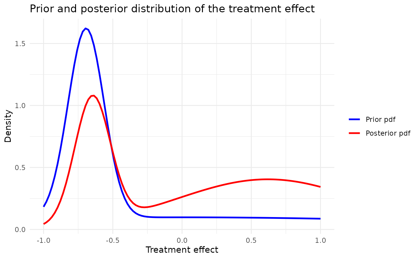
Posterior and prior pdf :

method_parameters$prior_weight <- 0.5

model <- Model$new()
model <- model$create(
  case_study_config = case_study_config,
  method = method,
  method_parameters = method_parameters,
  source_data = source_data
)

# Perform Bayesian inference based on observed target data.
model$inference(target_data = target_data)

## [1] "Success"

model$plot_pdfs(xmin = -1, xmax = 1, resolution = 100)

2026-10-03

Introduction

Set working directory, import functions and configurations

Define the method used (RMP) and the range of parameters considered

Create data objects

Inference

Plot results

Table summarizing the results

Posterior weight vs prior weight

Comparison with RBesT

Other treatment effect values in the target study

Plot results